Archive for the ‘Physics’ Category

Using Unambiguous Notation

October 19, 2007

I’ve mentioned their book the “Structure and Interpretation of Classical Mechanics” a couple times already; today I’d like to recommend that you read a wonderful short paper by Gerald Jay Sussman and Jack Wisdom, called “The Role of Programming in the Formulation of Ideas,” which helps explain why understanding physics and the other mathematical sciences can sometimes be so difficult. The basic point is that our notation is often an absolute mess, caused by the fact that we use equations like we use natural language, in a highly ambiguous way:

“It is necessary to present the science in the language of mathematics. Unfortunately, when we teach science we use the language of mathematics in the same way that we use our natural language. We depend upon a vast amount of shared knowledge and culture, and we only sketch an idea using mathematical idioms.”

The solution proposed is to develop notation that can be understood by computers, which do not tolerate ambiguity:

“One way to become aware of the precision required to unambiguously communicate a mathematical idea is to program it for a computer. Rather than using canned programs purely as an aid to visualization or numerical computation, we use computer programming in a functional style to encourage clear thinking. Programming forces one to be precise and formal, without being excessively rigorous. The computer does not tolerate vague descriptions or incomplete constructions. Thus the act of programming makes one keenly aware of one’s errors of reasoning or unsupported conclusions.”

Sussman and Wisdom then focus on one highly illuminating example, the Lagrange equations. These equations can be derived from the fundamental principle of least action. This principle tells you that if you have a classical system that begins in a configuration C1 at time t1 and arrives at a configuration C2 at time t2, the path it traces out between t1 and t2 will be the one that is consistent with the initial and final configurations and minimizes the integral over time of the Lagrangian for the system, where the Lagrangian is given by the kinetic energy minus the potential energy.

Physics textbooks tell us that if we apply the calculus of variations to the integral of the Lagrangian (called the “action”) we can derive that the true path satisfies the Lagrange equations, which are traditionally written as:

lagrange001.jpg

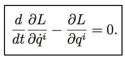
Here L is the Lagrangian, t is the time, annd qi are the coordinates of the system.

These equations (and many others like them) have confused and bewildered generations of physics students. What is the problem? Well, there are all sorts of fundamental problems in interpreting these equations, detailed in Sussman and Wisdom’s paper. As they point out, basic assumptions like whether a coordinate and its derivative are independent variables are not consistent within the same equation. And shouldn’t this equation refer to the path somewhere, since the Lagrange equations are only correct for the true path? I’ll let you read Sussman and Wisdom’s full laundry list of problems yourself. But let’s turn to the psychological effects of using such equations:

“Though such statements (and derivations that depend upon them) seem very strange to students, they are told that if they think about them harder they will understand. So the student must either come to the conclusion that he/she is dumb and just accepts it, or that the derivation is correct, with some appropriate internal rationalization. Students often learn to carry out these manipulations without really understanding what they are doing.”

Is this true? I believe it certainly is (my wife agrees: she gave up on mathematics, even though she always received excellent grades, because she never felt she truly understood). The students who learn to successfully rationalize such ambiguous equations, and forget about the equations that they can’t understand at all, are the ones who might go on to be successful physicists. Here’s an example, from the review of Sussman and Wisdom’s book by Piet Hut, a very well-regarded physicist who is now a professor at the Institute for Advanced Studies:

“… I went through the library in search of books on the variational principle in classical mechanics. I found several heavy tomes, borrowed them all, and started on the one that looked most attractive. Alas, it didn’t take long for me to realize that there was quite a bit of hand-waving involved. There was no clear definition of the procedure used for computing path integrals, let alone for the operations of differentiating them in various ways, by using partial derivatives and/or using an ordinary derivative along a particular path. And when and why the end points of the various paths had to be considered fixed or open to variation also was unclear, contributing to the overall confusion.

Working through the canned exercises was not very difficult, and from an instrumental point of view, my book was quite clear, as long as the reader would stick to simple examples. But the ambiguity of the presentation frustrated me, and I started scanning through other, even more detailed books. Alas, nowhere did I find the clarity that I desired, and after a few months I simply gave up. Like generations of students before me, I reluctantly accepted the dictum that ‘you should not try to understand quantum mechanics, since that will lead you astray for doing physics’, and going even further, I also gave up trying to really understand classical mechanics! Psychological defense mechanisms turned my bitter sense of disappointment into a dull sense of disenchantment.”

Sussman and Wisdom do show how the ambiguous conventional notation can be replaced with unambiguous notation that can even be used to program a computer. Because it’s new, it will feel alien at first; the Lagrange equations look like this:

functional002.jpg

It’s worth learning Sussman and Wisdom’s notation for the clarity it ultimately provides. It’s even more important to learn to always strive for clear understanding.

One final point: although mathematicians do often use notation that is superior to physicists’, they shouldn’t feel too smug; Sussman and Wisdom had similar things to say about differential geometry in this paper.

Advertisement

SICM on Mac OS X

October 17, 2007

“Structure and Interpretation of Classical Mechanics,” (SICM) by Gerald Jay Sussman and Jack Wisdom, with Meinhard Mayer, is a fascinating book, revisiting classical mechanics from the point of view that everything must be computationally explicit. I already mentioned the book in a previous post.

The book is available online, and all the software is freely available on-line as well. The software is written in Scheme, and a very extensive library called “scmutils” was developed to support computations in classical mechanics, including implementations of many symbolic and numerical algorithms.

I think that many scientists and programmers could find the “scmutils” library to be generally useful, even if they are not particularly interested in classical mechanics. If you are using the GNU/Linux operating system, there’s no problem in getting the library working. However, if you want to use it on Mac OS X (or Windows), the instructions leave the impression that it’s not possible, and Googling turned up some useful information, but no complete instructions, and also some people that seemed to be at a loss about how to do it.

Well, it is possible to get MIT-Scheme with the scmutils library running on Mac OS X (and you can probably modify my instructions to make it work on Windows too):

Click here for my instructions for running scmutils on Mac OS X.

Computing Free Energies

October 3, 2007

In my last post, I discussed phase transitions, and how computing the free energy for a model would let you work out the phase diagram. Today, I want to discuss in more detail some methods for computing free energies.

The most popular tool physicists use for computing free energies is “mean-field theory.” There seems to be at least one “mean-field theory” for every model in physics. When I was a graduate student, I became very unhappy with the derivations for mean-field theory, not because there were not any, but because there were too many! Every different book or paper had a different derivation, but I didn’t particularly like any of them, because none of them told you how to correct mean-field theory. That seemed strange because mean-field theory is known to only give approximate answers. It seemed to me that a proper derivation of mean-field theory would let you systematically correct the errors.

One paper really made me think hard about the problem; the famous 1977 “TAP” spin glass paper by Thouless, Anderson, and Palmer. They presented a mean-field free energy for the Sherrington-Kirkpatrick (SK) model of spin glasses by “fait accompli,” which added a weird “Onsager reaction term” to the ordinary free energy. This shocked me; maybe they were smart enough to write down free energies by fait accompli, but I needed some reliable mechanical method.

Since the Onsager reaction term had an extra power of 1/T compared to the ordinary energy term in the mean field theory, and the ordinary energy term had an extra power of 1/T compared to the entropy term, it looked to me like perhaps the TAP free energy could be derived from a high-temperature expansion. It would have to be a strange high-temperature expansion though, because it would need to be valid in the low-temperature phase!

Together with Antoine Georges, I worked out that the “high-temperature” expansion (it might better be thought of as a “weak interaction expansion”) could in fact be valid in a low-temperature phase, if one computed the free energy at fixed non-zero magnetization. This turned out to be the key idea; once we had it, it was just a matter of introducing Lagrange multipliers and doing some work to compute the details.

expansion001.jpg

It turned out that ordinary mean-field theory is just the first couple terms in a Taylor expansion. Computing more terms lets you systematically correct mean field theory, and thus compute the critical temperature of the Ising model, or any other quantities of interest, to better and better precision. The picture above is a figure from the paper, representing the expansion in a diagrammatic way.

We found out, after doing our computations but before submitting the paper, that in 1982 Plefka had already derived the TAP free energy for the SK model from that Taylor expansion, but for whatever reason, he had not gone beyond the Onsager correction term or noted that this was a technique that was much more general than the SK model for spin glasses, so nobody else had followed up using this approach.

If you want to learn more about this method for computing free energies, please read my paper (with Antoine Georges) “How to Expand Around Mean-Field Theory Using High Temperature Expansions,” or my paper “An Idiosyncratic Journey Beyond Mean Field Theory.”

This approach has some advantages and disadvantages compared with the belief propagation approach (and related Bethe free energy) which is much more popular in the electrical engineering and computer science communities. One advantage is that the free energy in the high-temperature expansion approach is just a function of simple one-node “beliefs” (the magnetizations), so it is computationally simpler to deal with than the Bethe free energy and belief propagation. Another advantage is that you can make systematic corrections; belief propagation can also be corrected with generalized belief propagation, but the procedure is less automatic. Disadvantages include the fact that the free energy is only exact for tree-like graphs if you add up an infinite number of terms, and the theory has not yet been formulated in an nice way for “hard” (infinite energy) constraints.

If you’re interested in quantum systems like e.g. the Hubbard model, the expansion approach has the advantage that it can also be applied to them; see my paper with Georges, or the lectures by Georges on his related “Dynamical Mean Field Theory,” or this recent paper by Plefka, who has returned to the subject more than 20 years after his original paper.

Also, if you’re interested in learning more about spin glasses or other disordered systems, or about other variational derivations for mean-field theory, please see this post.

Phase Transitions and Free Energies

October 2, 2007

Much of condensed matter and statistical physics is concerned with the explanation of phase transitions between different forms of matter. A familiar example is water, which has a transition from the solid phase of ice to the liquid phase, and then from the liquid phase to the gaseous phase of steam, as the temperature is increased.

In fact, many different materials have all sorts of exotic phases, as you vary the temperature, pressure, or composition of the material. Constructing “phase diagrams” which show what the different phases of a material should be as a function of the varying parameters is one of the main preoccupations of physicists.

How can these phase diagrams be constructed? Condensed matter physicists tend to follow the following algorithm. First, from arguments about the microscopic physics, construct a simple model of the local interactions of the molecules making up the material. Secondly, choose some method to approximately compute the “free energy” for that simple model. Finally, find the minima of the approximate free energy as a function of the adjustable parameters like the temperature. The phase diagram can be constructed by determining which phase has the lower free energy at each point in parameter space.

If the results disagree with experiment, your model is too simple or your approximation for the free energy is not good enough, so you need to improve one or the other or both; otherwise write up your paper and submit it for publication.

To illustrate, let’s consider magnetism. Although it is less familiar than the phase transition undergone by water, magnets also have a phase transition from a magnetized “frozen” phase at low temperature to an unmagnetized “paramagnetic” phase at high temperature.

The simplest model of magnetism is the Ising model. I’ve discussed this model before; to remind you, I’ll repeat the definition of the ferromagnetic Ising model: “In this model, there are spins at each node of a lattice, that can point ‘up’ or ‘down.’ Spins like to have their neighbors point in the same direction. To compute the energy of a configuration of spins, we look at all pairs of neighboring spins, and add an energy of -1 if the two spins point in the same direction, and an energy of +1 if the two spins point in opposite directions. Boltzmann’s law tells us that each configuration should have a probability proportional to the exp(-Energy[configuration] / T), where T is the temperature.”

Of course, as defined the Ising model is a mathematical object that can and has been studied mathematically independent of any relationship to physical magnets. Alternatively, the Ising model can be simulated on a computer.

Simulations (see this applet to experiment for yourself) show that at low temperatures (and if the dimensionality of the lattice is at least 2), the lattice of spins will over time tend to align so that they point together up more than down, or they all point down more than up. The natural symmetry between up and down is “broken.” At low temperatures one will find “domains” of spins pointing in the “wrong” direction, but these domains only last temporarily.

At high temperatures, on the other hand, each spin will typically fluctuate between pointing up and down, although again domains of like-pointing spins will form. The typical time for a spin to switch from pointing up to pointing down will increase as the temperature decreases, until it diverges towards infinity (as the size of the lattice approaches infinity) as one approaches the critical temperature from above.

Intuitively, the reason for this behavior is that at low temperature, the configurations where all the spins point in the same direction have a much lower energy, and thus a much higher probability, than other configurations. At high temperatures, all the configurations start having similar probabilities, and there are many more configurations that have equal numbers of up and down spins compared to the number of aligned configurations, so one typically sees the more numerous configurations.

This balance between energetic considerations (which make the spins align) and entropic considerations (which make the spins favor the more numerous unaligned configurations) is captured by the “free energy” F, which is given by the equation F=U-TS, where U is the average energy, S is the entropy, and T is the temperature. At low temperatures, the energy dominates the free energy, while at high temperatures, the entropy dominates.

All this intuition may be helpful, but like I said, the Ising model is a mathematical object, and we should be able to find approximation methods which let us precisely calculate the critical temperature. It would also be nice to be able to precisely calculate other interesting quantities, like the magnetization as a function of the temperature, or the susceptibility (which is the derivative of the magnetization with respect to an applied field) as a function of the temperature, or the specific heat (which is the derivative of the average energy with respect to the temperature) as a function of the temperature. All these quantities can be measured for real magnets, so if we compute them mathematically, we can judge how well the Ising model explains the magnets.

This post is getting a bit long, so I’ll wait until my next post to discuss in more detail some useful methods I have worked on for systematically and precisely computing free energies, and the other related quantities which can be derived from free energies.


The Hubbard Model: a Tutorial

September 9, 2007

Today, I will introduce a new kind of post at Nerd Wisdom, that I hope to do more of in the future: the tutorial. These posts will be a little more technical than ordinary posts, and will probably run a little longer as well. They are designed to give the intelligent and well-educated scientist an entry into a field for which he or she is not already a specialist.

When working with graduate-student interns, I find myself presenting these types of tutorials constantly. Unfortunately, this type of material is very hard to find in the literature, because it covers material that is too well-known to the specialist, while sometimes being beyond what is available in textbooks. Thus, there tends to be an artificial barrier to entry into new fields.

My first tutorial will cover the Hubbard Model. To keep this post to a reasonable length, I will just include the first part of the tutorial here.


I previously discussed high-temperature superconductivity in cuprates, and mentioned that the detailed mechanism is still controversial. However, what is widely agreed is that, as originally proposed by P.W. Anderson, a good model for these materials is the Hubbard Model (see this paper by Anderson for an entertaining and readable argument in favor of this point). And even if one doesn’t agree with that statement, the Hubbard Model is of enormous intrinsic interest, as perhaps the simplest model of interacting electrons on a lattice.

Despite its simplicity, physicists have not been able to solve for the behavior of the two or three-dimensional Hubbard model in the “thermodynamic limit” (for lattices with a very large number of sites and electrons). Coming up with a reliable approach to solving the Hubbard model has become a kind of holy grail of condensed matter theory.

Note that this is very different from the situation for the classical ferromagnetic Ising model, for which Onsager solved the two-dimensional version exactly in 1944 but where we do not have an exact solution in three dimensions. For the three-dimensional Ising model, we may not have an exact solution, but we understand extremely well the qualitative behavior, and can compute quantitative results to practically arbitrary accuracy. For the Hubbard model, we do not even have know what the qualitative behavior is for two or three dimensional lattices.

I will first describe the model in words, and then show you how to solve for the quantum statistical mechanics of the simplest non-trivial version of the model: the Hubbard model on a lattice with just two sites. I strongly believe that whenever you want to learn about a new algorithm or theory, you should start by solving, and understanding in detail, the smallest non-trivial version that you can construct.

The Full Tutorial

High-Temperature Superconductivity

September 7, 2007

In 1986, a new class of materials, called “cuprate superconductors,” was discovered by Karl Muller and Johannes Bednorz, which displayed superconductivity (the flow of electricity at zero resistance) at much higher temperatures than had ever previously been found. The discovery raised the possibility of materials that could super-conduct at ordinary room temperatures, which would clearly have great technological implications. Muller and Bednorz were awarded the Nobel Prize in Physics in 1987, which stands as the shortest period ever between a discovery and a Nobel prize.

I was a graduate student at Princeton when the news of high-temperature superconductivity broke, and my Ph.D. advisor was Philip W. Anderson, the 1977 Nobel Laureate in physics who at the time was already probably the most famous and respected condensed matter theorist in the world. (One recent study claimed to show that Anderson is the “most creative physicist in the world;” I found the method of the study highly dubious, but the conclusion is not unreasonable.) Anderson nearly immediately proposed a version of his “Resonating-Valence-Bond” theory for the superconductors, and trying to develop a complete theory has been his primary preoccupation ever since.

woodstock01_thumb.jpg

To give you an idea of the excitement in 1987, take a look at this article, looking back at the March 1987 meeting of the American Physical Society in New York City, characterized as the “Woodstock of Physics.”

I was at that meeting, and as one of Anderson’s students, I was definitely at the epicenter of the excitement, but I was actually rather turned off by the whole atmosphere, and I avoided working on the subject too seriously, focusing instead on neural networks and spin glass theory. (As I mentioned in this post, Anderson also made seminal contributions to those fields, and he let me work on whatever I was interested in.) Nevertheless, it was impossible to avoid being influenced, and I did eventually work on a few papers related to the theory of high-temperature superconductivity.

Sadly, the hopes for room temperature cuprate super-conductivity faded with time, and no cuprates have been discovered which super-conduct above 138 degrees Kelvin. And although our understanding of the materials has improved with time, there is still also considerable controversy about the mechanism causing the superconductivity.

See this post for more information about the Hubbard Model, which underlies the physics of the cuprates.

Consistent Quantum Theory

September 4, 2007

Quantum mechanics is a notoriously confusing and difficult subject, which is terribly unfortunate given its status as a fundamental theory of how the world works. When I was an undergraduate and graduate student of physics in the 1980’s, I was always unsatisfied with the way the subject was presented. We basically learned how to calculate solutions to certain problems, and there was an understanding that you were better off just avoiding the philosophical issues or the paradoxes surrounding the subject. After all, everybody knew that all the challenges raised by physicists as eminent as Einstein had ultimately been resolved experimentally in favor of the “Copenhagen interpretation.”

Still, there was a lot of weird stuff in the Copenhagen interpretation like the “collapse of the wave-function” caused by a measurement, or apparently non-local effects. What I wished existed was a clearly-defined and sensible set of “rules of the game” for using quantum mechanics. The need for such a set of rules has only increased with time with the advent of the field of quantum computing.

cover.gif

In his book, “Consistent Quantum Theory,” (the first 12 out of 27 chapters are available online) noted mathematical physicist Robert Griffiths provides the textbook I wished I had as a student. With contributions from Murray Gell-Mann, Roland Omnes, and James Hartle, Griffiths originated the “consistent history” approach to quantum mechanics which is explained in this book, .

The best summary of the approach can be obtained from the comparison Griffiths makes between quantum mechanics and the previous classical mechanics. Quantum mechanics differs from classical mechanics in the following ways:

1. Physical objects never posses a completely precise position or momentum.
2. The fundamental dynamical laws of physics are stochastic and not deterministic, so from the present state of the world one cannot infer a unique future (or past) course of events.
3. The principle of unicity does not hold: there is not a unique exhaustive description of a physical system or a physical process. Instead reality is such that it can be described in various alternative, incompatible ways, using descriptions which cannot be combined or compared.

It is the 3rd point which is the heart of the approach. In quantum mechanics, you are permitted to describe systems using one “consistent framework” or another, but you may not mix incompatible frameworks (basically frameworks using operators that don’t commute) together.

Griffiths uses toy models to illustrate the approach throughout the book, and provides resolutions for a large number of quantum paradoxes. He stresses that measurement plays no fundamental role in quantum mechanics, that wave function collapse is not a physical process, that quantum mechanics is a strictly local theory, and that reality exists independent of any observers. All of these points might seem philosphically natural and unremarkable, except for the fact that they contradict the standard Copenhagen interpretation.

This is a book that will take some commitment from the reader to understand, but it is the best explanation of quantum mechanics that I know of.

Richard Feynman

August 31, 2007

Richard Feynman has been one of my heroes, ever since the end of my freshman year at Harvard. After my last final exam, but before I headed home for the summer, I was able to sit in the beautiful Lowell House library, without any obligations, and just read chapters from his wonderful Lectures on Physics. After that there wasn’t much doubt in my mind about what I wanted to do with my life.

There’s a lot to say about Feynman, but I will restrict myself for now to a couple rather recent items which give a picture of the character of this remarkable man. First, there is this 1981 BBC Interview, recently released to the web, where you can see him briefly discuss a few of the things that were important to him.

images3.jpg

Secondly, if you haven’t read Perfectly Reasonable Deviations From the Beaten Track, the collection of his letters edited by his daughter Michelle Feynman that was published in 2005, you owe it to yourself to do so. I was skeptical at first that a book of letters, even those of Feynman, could be very interesting, but I wound up reading every word.

Let me just give you one example of a pair of letters from 1964:

Dear Professor Feynman,

Dr Marvin Chester is presently under consideration for promotion to the Associate Professorship in our department. I would be very grateful for a letter from you evaluating his stature as a physicist. May I thank you in advance for your cooperation in this matter.

Sincerely,
D.S Saxon
Chairman
Dick: Sorry to bother you, but we really need this sort of thing.
David S.

Dr. D.S. Saxon, Chairman
Department of Physics
University of California, Los Angeles
Los Angeles, California

Dear David:

This is in answer to your request for a letter evaluating Dr. Marvin Chester’s research contributions and his stature as a physicist.

What’s the matter with you fellows, he has been right there the past few years–can’t you “evaluate” him best yourself? I can’t do much better than the first time you asked me, a few years ago when he was working here, because I haven’t followed his research in detail. At that time, I was very much impressed with his originality, his ablity to carry a theoretical argument to its practical, experimental conclusions, and to design and perform the key experiments. Rarely have I met that combination in such good balance in a student. Was I wrong? How has he been making out?

Sincerely yours,
R.P. Feynman

The above letter stands out in the files of recommendations. After this time, any request for a recommendation by the facility where the scientist was working was refused.

Edit: In the comments below, Shimon Schocken recommends Feynman’s “QED.” I thought of this book after finishing this post. It’s an amazing work. In it, Feynman gives a popular account (you don’t need any physics background to follow it) of his theory of quantum electrodynamics, for which he won the Nobel Prize. But it’s a popular account that makes no compromises in its scientific accuracy. The other books recommended in the comments (“Six Easy Pieces” and “Surely You’re Joking”) are also definitely great books, but “QED” is somehow often overlooked, even though it is the book that Feynman himself recommended to those interested in his work.