Archive for the ‘Statistical Physics’ Category

Computing Free Energies

October 3, 2007

In my last post, I discussed phase transitions, and how computing the free energy for a model would let you work out the phase diagram. Today, I want to discuss in more detail some methods for computing free energies.

The most popular tool physicists use for computing free energies is “mean-field theory.” There seems to be at least one “mean-field theory” for every model in physics. When I was a graduate student, I became very unhappy with the derivations for mean-field theory, not because there were not any, but because there were too many! Every different book or paper had a different derivation, but I didn’t particularly like any of them, because none of them told you how to correct mean-field theory. That seemed strange because mean-field theory is known to only give approximate answers. It seemed to me that a proper derivation of mean-field theory would let you systematically correct the errors.

One paper really made me think hard about the problem; the famous 1977 “TAP” spin glass paper by Thouless, Anderson, and Palmer. They presented a mean-field free energy for the Sherrington-Kirkpatrick (SK) model of spin glasses by “fait accompli,” which added a weird “Onsager reaction term” to the ordinary free energy. This shocked me; maybe they were smart enough to write down free energies by fait accompli, but I needed some reliable mechanical method.

Since the Onsager reaction term had an extra power of 1/T compared to the ordinary energy term in the mean field theory, and the ordinary energy term had an extra power of 1/T compared to the entropy term, it looked to me like perhaps the TAP free energy could be derived from a high-temperature expansion. It would have to be a strange high-temperature expansion though, because it would need to be valid in the low-temperature phase!

Together with Antoine Georges, I worked out that the “high-temperature” expansion (it might better be thought of as a “weak interaction expansion”) could in fact be valid in a low-temperature phase, if one computed the free energy at fixed non-zero magnetization. This turned out to be the key idea; once we had it, it was just a matter of introducing Lagrange multipliers and doing some work to compute the details.

expansion001.jpg

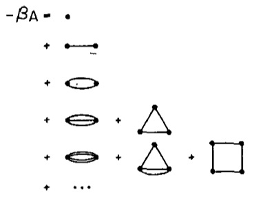
It turned out that ordinary mean-field theory is just the first couple terms in a Taylor expansion. Computing more terms lets you systematically correct mean field theory, and thus compute the critical temperature of the Ising model, or any other quantities of interest, to better and better precision. The picture above is a figure from the paper, representing the expansion in a diagrammatic way.

We found out, after doing our computations but before submitting the paper, that in 1982 Plefka had already derived the TAP free energy for the SK model from that Taylor expansion, but for whatever reason, he had not gone beyond the Onsager correction term or noted that this was a technique that was much more general than the SK model for spin glasses, so nobody else had followed up using this approach.

If you want to learn more about this method for computing free energies, please read my paper (with Antoine Georges) “How to Expand Around Mean-Field Theory Using High Temperature Expansions,” or my paper “An Idiosyncratic Journey Beyond Mean Field Theory.”

This approach has some advantages and disadvantages compared with the belief propagation approach (and related Bethe free energy) which is much more popular in the electrical engineering and computer science communities. One advantage is that the free energy in the high-temperature expansion approach is just a function of simple one-node “beliefs” (the magnetizations), so it is computationally simpler to deal with than the Bethe free energy and belief propagation. Another advantage is that you can make systematic corrections; belief propagation can also be corrected with generalized belief propagation, but the procedure is less automatic. Disadvantages include the fact that the free energy is only exact for tree-like graphs if you add up an infinite number of terms, and the theory has not yet been formulated in an nice way for “hard” (infinite energy) constraints.

If you’re interested in quantum systems like e.g. the Hubbard model, the expansion approach has the advantage that it can also be applied to them; see my paper with Georges, or the lectures by Georges on his related “Dynamical Mean Field Theory,” or this recent paper by Plefka, who has returned to the subject more than 20 years after his original paper.

Also, if you’re interested in learning more about spin glasses or other disordered systems, or about other variational derivations for mean-field theory, please see this post.

Phase Transitions and Free Energies

October 2, 2007

Much of condensed matter and statistical physics is concerned with the explanation of phase transitions between different forms of matter. A familiar example is water, which has a transition from the solid phase of ice to the liquid phase, and then from the liquid phase to the gaseous phase of steam, as the temperature is increased.

In fact, many different materials have all sorts of exotic phases, as you vary the temperature, pressure, or composition of the material. Constructing “phase diagrams” which show what the different phases of a material should be as a function of the varying parameters is one of the main preoccupations of physicists.

How can these phase diagrams be constructed? Condensed matter physicists tend to follow the following algorithm. First, from arguments about the microscopic physics, construct a simple model of the local interactions of the molecules making up the material. Secondly, choose some method to approximately compute the “free energy” for that simple model. Finally, find the minima of the approximate free energy as a function of the adjustable parameters like the temperature. The phase diagram can be constructed by determining which phase has the lower free energy at each point in parameter space.

If the results disagree with experiment, your model is too simple or your approximation for the free energy is not good enough, so you need to improve one or the other or both; otherwise write up your paper and submit it for publication.

To illustrate, let’s consider magnetism. Although it is less familiar than the phase transition undergone by water, magnets also have a phase transition from a magnetized “frozen” phase at low temperature to an unmagnetized “paramagnetic” phase at high temperature.

The simplest model of magnetism is the Ising model. I’ve discussed this model before; to remind you, I’ll repeat the definition of the ferromagnetic Ising model: “In this model, there are spins at each node of a lattice, that can point ‘up’ or ‘down.’ Spins like to have their neighbors point in the same direction. To compute the energy of a configuration of spins, we look at all pairs of neighboring spins, and add an energy of -1 if the two spins point in the same direction, and an energy of +1 if the two spins point in opposite directions. Boltzmann’s law tells us that each configuration should have a probability proportional to the exp(-Energy[configuration] / T), where T is the temperature.”

Of course, as defined the Ising model is a mathematical object that can and has been studied mathematically independent of any relationship to physical magnets. Alternatively, the Ising model can be simulated on a computer.

Simulations (see this applet to experiment for yourself) show that at low temperatures (and if the dimensionality of the lattice is at least 2), the lattice of spins will over time tend to align so that they point together up more than down, or they all point down more than up. The natural symmetry between up and down is “broken.” At low temperatures one will find “domains” of spins pointing in the “wrong” direction, but these domains only last temporarily.

At high temperatures, on the other hand, each spin will typically fluctuate between pointing up and down, although again domains of like-pointing spins will form. The typical time for a spin to switch from pointing up to pointing down will increase as the temperature decreases, until it diverges towards infinity (as the size of the lattice approaches infinity) as one approaches the critical temperature from above.

Intuitively, the reason for this behavior is that at low temperature, the configurations where all the spins point in the same direction have a much lower energy, and thus a much higher probability, than other configurations. At high temperatures, all the configurations start having similar probabilities, and there are many more configurations that have equal numbers of up and down spins compared to the number of aligned configurations, so one typically sees the more numerous configurations.

This balance between energetic considerations (which make the spins align) and entropic considerations (which make the spins favor the more numerous unaligned configurations) is captured by the “free energy” F, which is given by the equation F=U-TS, where U is the average energy, S is the entropy, and T is the temperature. At low temperatures, the energy dominates the free energy, while at high temperatures, the entropy dominates.

All this intuition may be helpful, but like I said, the Ising model is a mathematical object, and we should be able to find approximation methods which let us precisely calculate the critical temperature. It would also be nice to be able to precisely calculate other interesting quantities, like the magnetization as a function of the temperature, or the susceptibility (which is the derivative of the magnetization with respect to an applied field) as a function of the temperature, or the specific heat (which is the derivative of the average energy with respect to the temperature) as a function of the temperature. All these quantities can be measured for real magnets, so if we compute them mathematically, we can judge how well the Ising model explains the magnets.

This post is getting a bit long, so I’ll wait until my next post to discuss in more detail some useful methods I have worked on for systematically and precisely computing free energies, and the other related quantities which can be derived from free energies.


Two Draft Books

September 13, 2007

If you’re interested in learning about statistical mechanics, graphical models, information theory, error-correcting codes, belief propagation, constraint satisfaction problems, or the connections between all those subjects, you should know about a couple of books that should be out soon, but for which you can already download extensive draft versions.

The first is Information, Physics, and Computation by Marc Mézard and Andrea Montanari.

The second is Modern Coding Theory by Tom Richardson and Ruediger Urbanke.

I also recommend the tutorial on Modern Coding Theory: the Statistical Mechanics and Computer Science Points of View, by Montanari and Urbanke, from the lectures they gave at the 2006 Les Houches summer school.

The Hubbard Model: a Tutorial

September 9, 2007

Today, I will introduce a new kind of post at Nerd Wisdom, that I hope to do more of in the future: the tutorial. These posts will be a little more technical than ordinary posts, and will probably run a little longer as well. They are designed to give the intelligent and well-educated scientist an entry into a field for which he or she is not already a specialist.

When working with graduate-student interns, I find myself presenting these types of tutorials constantly. Unfortunately, this type of material is very hard to find in the literature, because it covers material that is too well-known to the specialist, while sometimes being beyond what is available in textbooks. Thus, there tends to be an artificial barrier to entry into new fields.

My first tutorial will cover the Hubbard Model. To keep this post to a reasonable length, I will just include the first part of the tutorial here.


I previously discussed high-temperature superconductivity in cuprates, and mentioned that the detailed mechanism is still controversial. However, what is widely agreed is that, as originally proposed by P.W. Anderson, a good model for these materials is the Hubbard Model (see this paper by Anderson for an entertaining and readable argument in favor of this point). And even if one doesn’t agree with that statement, the Hubbard Model is of enormous intrinsic interest, as perhaps the simplest model of interacting electrons on a lattice.

Despite its simplicity, physicists have not been able to solve for the behavior of the two or three-dimensional Hubbard model in the “thermodynamic limit” (for lattices with a very large number of sites and electrons). Coming up with a reliable approach to solving the Hubbard model has become a kind of holy grail of condensed matter theory.

Note that this is very different from the situation for the classical ferromagnetic Ising model, for which Onsager solved the two-dimensional version exactly in 1944 but where we do not have an exact solution in three dimensions. For the three-dimensional Ising model, we may not have an exact solution, but we understand extremely well the qualitative behavior, and can compute quantitative results to practically arbitrary accuracy. For the Hubbard model, we do not even have know what the qualitative behavior is for two or three dimensional lattices.

I will first describe the model in words, and then show you how to solve for the quantum statistical mechanics of the simplest non-trivial version of the model: the Hubbard model on a lattice with just two sites. I strongly believe that whenever you want to learn about a new algorithm or theory, you should start by solving, and understanding in detail, the smallest non-trivial version that you can construct.

The Full Tutorial

Algorithms for Physics

August 14, 2007


smac_cover.jpg

Much of my own work is at the intersection of statistical mechanics and algorithms, in particular understanding and developing new algorithms using ideas originating in statistical mechanics. Werner Krauth also works at the intersection of the two fields, but coming from a very different angle: he is a leading expert on the development and application of algorithms to compute and understand the properties of physical systems.

In his recently published book, “Statistical Mechanics: Algorithms and Computations,” targeted at advanced undergraduates or graduate students, he covers a very wide range of interesting algorithms. To give you an idea of the coverage, I’ll just list the chapters: “Monte Carlo methods,” “Hard disks and spheres,” “Density matrices and path integrals,” “Bosons,” “Order and disorder in spin systems, “Entropic forces,”and “Dynamic Monte Carlo methods.”

Krauth’s presentation is leavened by his humor, and he often uses the results obtained using his algorithms to make surprising points about physics that would otherwise be hard to convey.

I am often asked by computer science or electrical engineering scientists and researchers for good introductions to physics, and particularly statistical mechanics, and I’m now happy to be able to recommend this book.

images.jpg

Specifying physics explicitly in terms of algorithms, as Krauth does, gives a very concrete basis for understanding concepts that can otherwise seem terribly abstract. Gerald Sussman and Jack Wisdom make this point in the preface of their already classic book (which is available online) “Structure and Interpretation of Classical Mechanics”:

“Computational algorithms are used to communicate precisely some of the methods used in the analysis of dynamical phenomena. Expressing the methods of variational mechanics in a computer language forces them to be unambiguous and computationally effective. Computation requires us to be precise about the representation of mechanical and geometric notions as computational objects and permits us to represent explicitly the algorithms for manipulating these objects. Also, once formalized as a procedure, a mathematical idea becomes a tool that can be used directly to compute results.”

But while Sussman and Wisdom’s book focuses in great detail on classical mechanics, Krauth’s book covers more broadly subjects in classical mechanics, statistical mechanics, quantum mechanics, and even quantum statistical mechanics. Another difference is that Sussman and Wisdom specify their algorithms in executable Scheme code, while Krauth uses pseudo-code. Of course, both choices have their advantages, just as both of these books are worth your time.

Lectures on Disordered Systems

August 12, 2007

Many physicists study “disordered systems,” such as materials like glasses where the molecules making up the material are arranged randomly in space, in contrast to crystals, where all the particles are arranged in beautiful repeating patterns.

The symmetries of crystals make them much easier to analyze than glasses, and new theoretical methods had to be invented before physicists could make any headway in computing the properties of disordered systems. Those methods have turned out to be closely connected to approaches, such as the “belief propagation” algorithm, that are widely used in computer science, artificial intelligence, and communications theory, with the result that physicists and computer scientists today regularly exchange new ideas and results across their disciplines.

Returning to the physics of disordered systems, physicists began working on the problem in the 1970’s by considering the problem of disordered magnets (also called “spin glasses”). My Ph.D. thesis advisor, Philip W. Anderson summarized the history as follows:

“In 1975 S.F. (now Sir Sam) Edwards and I wrote down the “replica” theory of the phenomenon I had earlier named “spin glass”, followed up in ’77 by a paper of D.J. Thouless, my student Richard Palmer, and myself. A brilliant further breakthrough by G. Toulouse and G. Parisi led to a full solution of the problem, which turned out to entail a new form of statistical mechanics of wide applicability in fields as far apart as computer science, protein folding, neural networks, and evolutionary modelling, to all of which directions my students and/or I contributed.”

csss_us.jpg

In 1992, I presented five lectures on “Quenched Disorder: Understanding Glasses Using a Variational Principle and the Replica Method” at a Santa Fe Institute summer school on complex systems. The lectures were published in a book edited by Lynn Nadel and Daniel Stein, but that book is very hard to find, and I think that these lectures are still relevant, so I’m posting them here. As I say in the introduction, “I will discuss technical subjects, but I will try my best to introduce all the technical material in as gentle and comprehensible a way as possible, assuming no previous exposure to the subject of these lectures at all.”

The first lecture is an introduction to the basics of statistical mechanics. It introduces magnetic systems and particle systems, and describes how to exactly solve non-interacting magnetic systems and particle systems where the particles are connected by springs.

The second lecture introduces the idea of variational approaches. Roughly speaking, the idea of a variational approach is to construct an approximate but exactly soluble system that is as close as possible to the system you are interested in. The grandly titled “Gaussian variational method” is the variational method that tries to find the set of particles and springs that best approximates an interacting particle system. I describe in this second lecture how the Gaussian variational method can be applied to heteropolymers like proteins.

The next three lectures cover the replica method, and combine it with the variational approach. The replica method is highly intricate mathematically. I learned it at the feet of the masters during my two years at the Ecole Normale Superieure (ENS) in Paris. In particular, I was lucky to work with Jean-Philippe Bouchaud, Antoine Georges, and Marc Mezard, who taught me what I knew. I thought it unfortunate that there wasn’t a written tutorial on the replica method, so the result were these lectures. Marc told me that for years afterwards they were given to new students of the replica method at the ENS.

Nowadays, the replica method is a little less popular than it used to be, mostly because it is all about computing averages of quantities over many samples of systems that are disordered according to some probability distribution. While those averages are very useful in physics, they are somewhat less important in computer science, where you usually just want an algorithm to deal with the one disordered system in front of you, rather than an average over all the possible disordered systems.

Santa Fe Institute Lectures

Generalized Belief Propagation

August 5, 2007

In 2002, I gave a lecture at the Mathematical Sciences Research Institute on the work I did, together with Bill Freeman and Yair Weiss on Generalized Belief Propagation, and the correspondence between free energy approximations and message passing algorithms. The lecture is available as a streaming video, together with a pdf for the slides, here.

It’s worth mentioning that there are many other interesting research lectures available in MSRI’s video archive, and that the more recent ones are of higher production quality.

Here is our most recent and comprehensive paper on this subject, published in the July 2005 issue of IEEE Transactions on Information Theory, which gives many additional details compared to the lecture: MERL TR2004-040.

If that paper is too difficult, you should probably start with this earlier paper, which was more tutorial in nature: MERL TR2001-22.

If you’re looking for generalized belief propagation software, your best bet is this package written by Yair’s student Talya Meltzer.

P.S.: I realized I haven’t told those of you who don’t know anything about it what generalized belief propagation is. Well, one answer is to that is look at the above material! But here’s a little background text that I’ve copied from my research statement to explain why you might be interested:

Most of my current research involves the application of statistical methods to “inference” problems. Some important fields which are dominated by the issue of inference are computer vision, speech recognition, natural language processing, error-control coding and digital communications. Essentially, any time you are receiving a noisy signal, and need to infer what is really out there, you are dealing with an inference problem.

A productive way to deal with an inference problem is to formalize it as a problem of computing probabilities in a “graphical model.” Graphical models, which are referred to in various guises as “Markov random fields,” “Bayesian networks,” or “factor graphs,” provide a statistical framework to encapsulate our knowledge of a system and to infer from incomplete information.

Physicists who use the techniques of statistical mechanics to study the behavior of disordered magnetic spin systems are actually studying a mathematically equivalent problem to the inference problem studied by computer scientists or electrical engineers, but with different terminology, goals, and perspectives. My own research has focused on the surprising relationships between methods that are used in these communities, and on powerful new techniques and algorithms, such as Generalized Belief Propagation, that can be understood using those relationships.

I’ll tell you more in future posts; I promise.

David MacKay’s “Information Theory, Inference, and Learning Algorithms”

August 1, 2007

sept2003cover25.gif

This is an easy book for me to recommend. David J.C. MacKay is a professor in the physics department of Cambridge University, and he is a polymath who has made important contributions in a wide variety of fields. This textbook is an excellent introduction to modern error-correcting codes, compression, statistical physics, and neural networks. It is tied together by a recurring appeal to the power of Bayesian methods.

David wrote this book over the course of many years, publishing his drafts on the web. You can still view the entire book on the web here. But the book is very inexpensive; unless you’re very poor, you’ll really want to buy a copy.

As Bob McEliece (a professor at Caltech and Shannon medalist) wrote, “you’ll want two copies of this astonishing book, one for the office and one for the fireside at home.” I know this is true because I actually have two copies; I bought my own copy as soon as the book was published, and then found that David had kindly sent me a copy.